FILTERS IN ELECTRONICS AND THEIR CLASSSIFICATION, FILTER TYPES
Table of Contents
FILTERS INTRODUCTION:
Filters of some sort are essential to the operation of most electronic circuits. It is therefore in the interest of anyone involved in electronic circuit design to have the ability to develop filter circuits capable of meeting a given set of specifications. Unfortunately, many in the electronics field are uncomfortable with the subject, whether due to a lack of familiarity with it, or a reluctance to grapple with the mathematics involved in a complex filter design. This Application Note is intended to serve as a very basic introduction to some of the fundamental concepts and terms associated with filters. It will not turn a novice into a filter designer, but it can serve as a starting point for those wishing to learn more about filter design.
Filters and Signals: What Does a Filter Do?
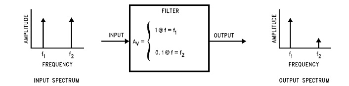
In circuit theory, a filter is an electrical network that alters the amplitude and/or phase characteristics of a signal with respect to frequency. Ideally, a filter will not add new frequencies to the input signal, nor will it change the component frequencies of that signal, but it will change the relative amplitudes of the various frequency components and/or their phase relationships. Filters are often used in electronic systems to emphasize signals in certain frequency ranges and reject signals in other frequency ranges. Such a filter has a gain which is dependent on signal frequency. As an example, consider a situation where a useful signal at frequency f1 has been contaminated with an unwanted signal at f2. If the contaminated signal is passed through a circuit (Figure 1) that has very low gain at f2 compared to f1, the undesired signal can be removed, and the useful signal will remain. Note that in the case of this simple example, we are not concerned with the gain of the filter at any frequency other than f1 and f2. As long as f2 is sufficiently attenuated relative to f1, the performance of this filter will be satisfactory. In general, however, a filter’s gain may be specified at several different frequencies, or over a band of frequencies. Since filters are defined by their frequency-domain effects on signals, it makes sense that the most useful analytical and graphical descriptions of filters also fall into the frequency domain. Thus, curves of gain vs. frequency and phase vs. frequency are commonly used to illustrate filter characteristics, and the most widely-used mathematical tools are based in the frequency domain.
The frequency-domain behavior of a filter is described mathematically in terms of its transfer function or network function. This is the ratio of the Laplace transforms of its output and input signals. The voltage transfer function H(s) of a filter can therefore be written as:
H(s) = (VOUT(s) / VIN(s)
Where VIN(s) and VOUT(s) are the input and output signal voltages and s is the complex frequency variable. The transfer function defines the filter’s response to any arbitrary input signal, but we are most often concerned with its effect on continuous sine waves. Especially important is the magnitude of the transfer function as a function of frequency, which indicates the effect of the filter on the amplitudes of sinusoidal signals at various frequencies. Knowing the transfer function magnitude (or gain) at each frequency allows us to determine how well the filter can distinguish between signals at different frequencies. The transfer function magnitude versus frequency is called the amplitude response or sometimes, especially in audio applications, the frequency response.
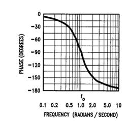
Similarly, the phase response of the filter gives the amount of phase shift introduced in sinusoidal signals as a function of frequency. Since a change in phase of a signal also represents a change in time, the phase characteristics of a filter become especially important when dealing with complex signals where the time relationships between signal components at different frequencies are critical. By replacing the variables in (1) with j0, where j is equal to 1, and 0 is the radian frequency, we can find the filter’s effect on the magnitude and phase of the input signal.
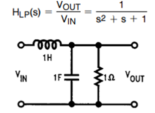
As an example, the network of Figure 2 has the transfer function:
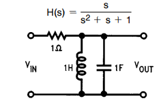
This is a 2nd order system. The order of a filter is the highest power of the variable s in its transfer function. The order of a filter is usually equal to the total number of capacitors and inductors in the circuit. (A capacitor built by combining two or more individual capacitors is still one capacitor.) Higher-order filters will obviously be more expensive to build, since they use more components, and they will also be more complicated to design. However, higher-order filters can more effectively discriminate between signals at different frequencies.
Before actually calculating the amplitude response of the network, we can see that at very low frequencies (small values of s), the numerator becomes very small, as do the first two terms of the denominator. Thus, as s approaches zero, the numerator approaches zero, the denominator approaches one, and H(s) approaches zero. Similarly, as the input frequency approaches infinity, H(s) also becomes progressively smaller, because the denominator increases with the square of frequency while the numerator increases linearly with frequency. Therefore, H(s) will have its maximum value at some frequency between zero and infinity, and will decrease at frequencies above and below the peak. To find the magnitude of the transfer function, replace s with j0 to yield:
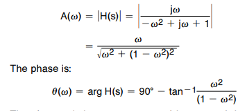
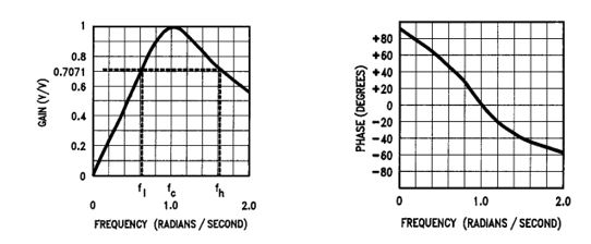
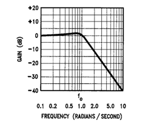
The above relations are expressed in terms of the radian frequency 0, in units of radians/second. A sinusoid will complete one full cycle in 2q radians. Plots of magnitude and phase versus radian frequency are shown in Figure 3. When we are more interested in knowing the amplitude and phase response of a filter in units of Hz (cycles per second), we convert from radian frequency using 0 e 2Õf, where f is the frequency in Hz. The variables f and 0 are used more or less interchangeably, depending upon which is more appropriate or convenient for a given situation.
Figure 3(a) shows that, as we predicted, the magnitude of the transfer function has a maximum value at a specific frequency (00) between 0 and infinity, and falls off on either side of that frequency. A filter with this general shape is known as a band-pass filter because it passes signals falling within a relatively narrow band of frequencies and attenuates signals outside of that band. The range of frequencies passed by a filter is known as the filter’s pass band. Since the amplitude response curve of this filter is fairly smooth, there are no obvious boundaries for the pass band. Often, the pass band limits will be defined by system requirements. A system may require, for example, that the gain variation between 400 Hz and 1.5 kHz be less than 1 dB. This specification would effectively define the pass band as 400 Hz to 1.5 kHz. In other cases though, we may be presented with a transfer function with no pass band limits specified. In this case, and in any other case with no explicit pass band limits, the pass band limits are usually assumed to be the frequencies where the gain has dropped by 3 decibels (to 02/2 or 0.707 of its maximum voltage gain). These frequencies are therefore called the b3 dB frequencies or the cutoff frequencies. However, if a pass band gain variation (i.e., 1 dB) is specified, the cutoff frequencies will be the frequencies at which the maximum gain variation specification is exceeded.
The precise shape of a band-pass filter’s amplitude response curve will depend on the particular network, but any 2nd order band-pass response will have a peak value at the filter’s center frequency. The center frequency is equal to the geometric mean of the -3 dB frequencies.
Another quantity used to describe the performance of a filter is the filter’s ‘‘Q’’. This is a measure of the ‘‘sharpness’’ of the amplitude response. The Q of a band-pass filter is the ratio of the center frequency to the difference between the -3 dB frequencies (also known as the b3 dB bandwidth).
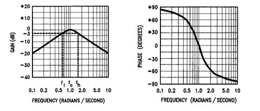
When evaluating the performance of a filter, we are usually interested in its performance over ratios of frequencies. Thus we might want to know how much attenuation occurs at twice the center frequency and at half the center frequency. (In the case of the 2nd-order band pass above, the attenuation would be the same at both points). It is also usually desirable to have amplitude and phase response curves that cover a wide range of frequencies. It is difficult to obtain a useful response curve with a linear frequency scale if the desire is to observe gain and phase over wide frequency ratios. For example, if f0 e 1 kHz, and we wish to look at response to 10 kHz, the amplitude response peak will be close to the left-hand side of the frequency scale. Thus, it would be very difficult to observe the gain at 100 Hz, since this would represent only 1% of the frequency axis. A logarithmic frequency scale is very useful in such cases, as it gives equal weight to equal ratios of frequencies. Since the range of amplitudes may also be large, the amplitude scale is usually expressed in decibels (20loglH (j0) l). Figure 4 shows the curves of Figure 3 with logarithmic frequency scales and a decibel amplitude scale. Note the improved symmetry in the curves of Figure 4 relative to those of Figure 3.
The Basic Filter Types
BAND PASS FILTER:-
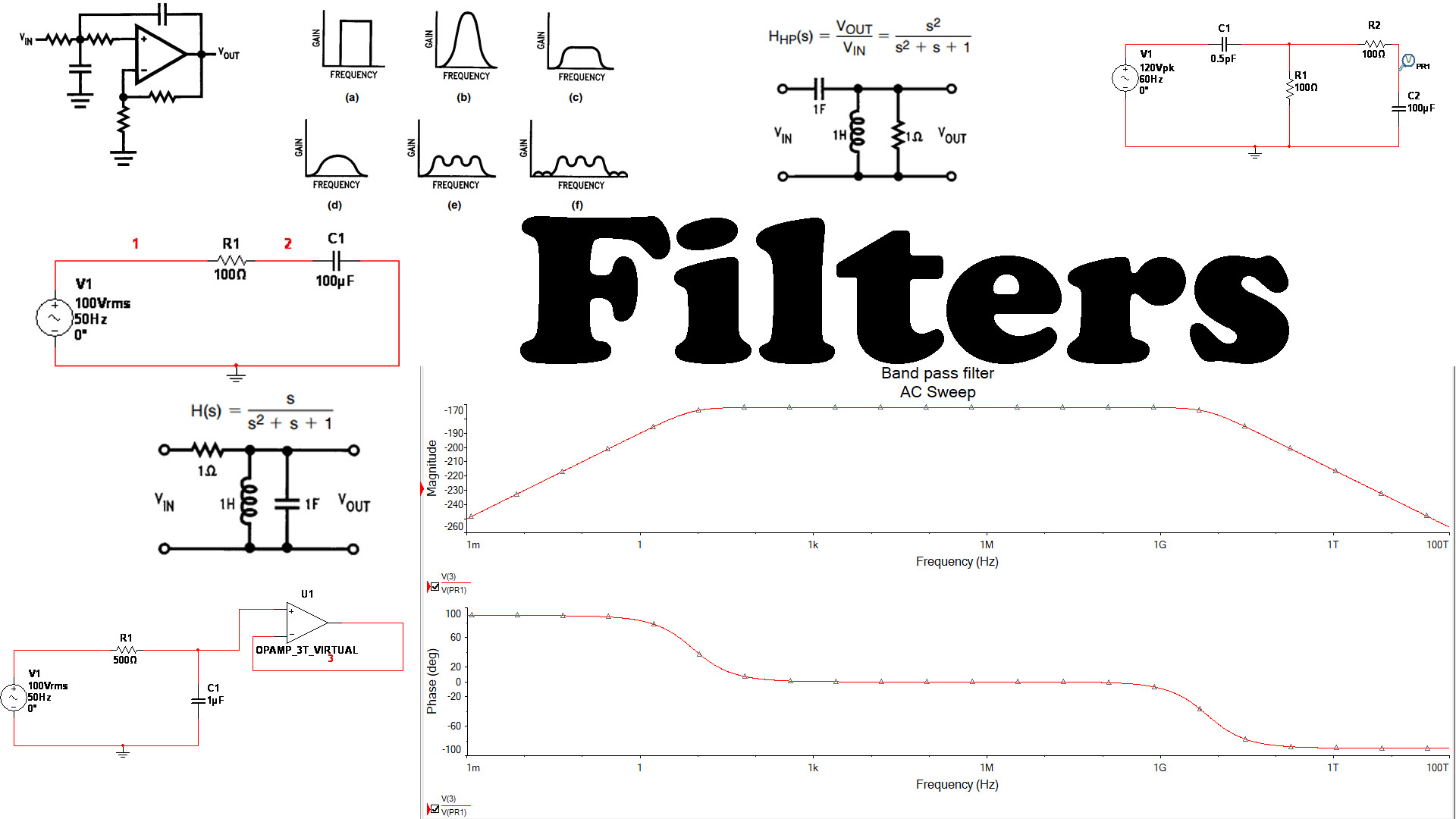
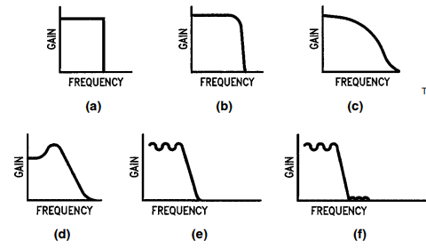
There are five basic filter types (band pass, notch, low-pass, high-pass, and order filters). The filter used in the example in the previous section was a band pass. The number of possible band pass response characteristics is infinite, but they all share the same basic form. Several examples of band pass amplitude response curves are shown in Figure 5. The curve in 5(a) is what might be called an ‘‘ideal’’ band pass response, with absolutely constant gain within the pass band, zero gain outside the pass band, and an abrupt boundary between the two. This response characteristic is impossible to realize in practice, but it can be approximated to varying degrees of accuracy by real filters. Curves (b) through (f) are examples of a few band pass amplitude response curves that approximate the ideal curves with varying degrees of accuracy. Note that while some band pass responses are very smooth, other have ripple (gain variations in their pass bands. Other have ripple in their stop bands as well. The stop band is the range of frequencies over which unwanted signals are attenuated. Band pass filters have two stop bands, one above and one below the pass band.

Just as it is difficult to determine by observation exactly where the pass band ends, the boundary of the stop band is also seldom obvious. Consequently, the frequency at which a stop band begins is usually defined by the requirements of a given system for example, a system specification might require that the signal must be attenuated at least 35 dB at 1.5 kHz. This would define the beginning of a stop band at 1.5 kHz. The rate of change of attenuation between the pass band and the stop band also differs from one filter to the next. The slope of the curve in this region depends strongly on the order of the filter, with higher-order filters having steeper cutoff slopes. The attenuation slope is usually expressed in dB/octave (an octave is a factor of 2 in frequency) or dB/ decade (a decade is a factor of 10 in frequency). Band pass filters are used in electronic systems to separate a signal at one frequency or within a band of frequencies from signals at other frequencies. In 1.1 an example was given of a filter whose purpose was to pass a desired signal at frequency f1, while attenuating as much as possible an unwanted signal at frequency f2. This function could be performed by an appropriate band pass filter with center frequency f1. Such a filter could also reject unwanted signals at other frequencies outside of the pass band, so it could be useful in situations where the signal of interest has been contaminated by signals at a number of different frequencies.
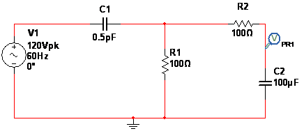
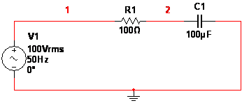
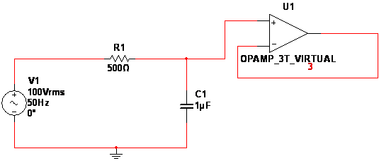
Band pass filter circuit diagram
Wire up the Circuit as shown below.
Download Band Pass Filter Simulation:
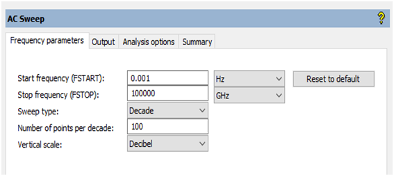
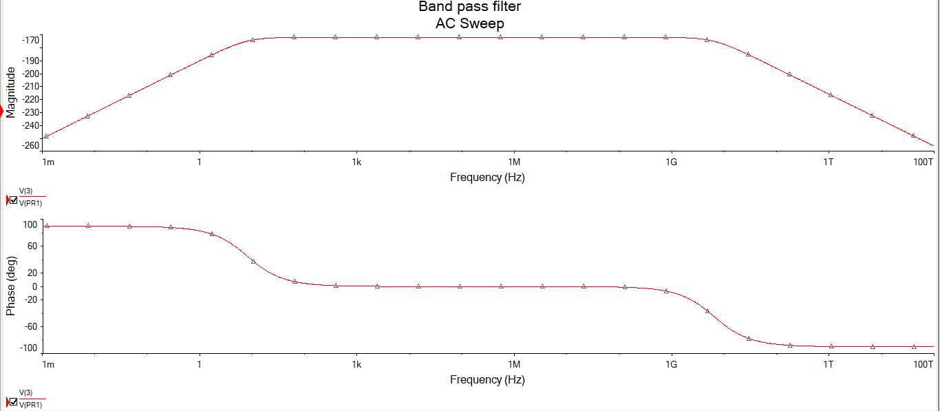
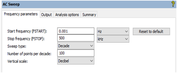
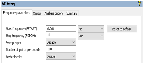
Analysis Parameters for Band pass filter
Select the Simulation and set it to Ac Sweep, set the analysis parameters
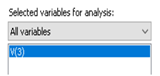
Now select the output variables meters as required in this case
Press F5 and observe the simulation result of Circuit
LOW PASS FILTER
A third filter type is the low-pass. A low-pass filter passes low frequency signals, and rejects signals at frequencies above the filter’s cutoff frequency. If the components of our example circuit are rearranged as in Figure 8, the resultant transfer function is:
It is easy to see by inspection that this transfer function has more gain at low frequencies than at high frequencies. As omega approaches 0, HLP approaches 1; as omega approaches infinity, HLP approaches 0. Amplitude and phase response curves are shown in Figure 9, with an assortment of possible amplitude response curves in Figure 10. Note that the various approximations to the unrealizable ideal low-pass amplitude characteristics take different forms, some being monotonic (always having a negative slope), and others having ripple in the pass band and/or stop band
Low-pass filters are used whenever high frequency components must be removed from a signal. An example might be in a light-sensing instrument using a photodiode. If light levels are low, the output of the photodiode could be very small, allowing it to be partially obscured by the noise of the sensor and its amplifier, whose spectrum can extend to very high frequencies. If a low-pass filter is placed at the output of the amplifier, and if its cutoff frequency is high enough to allow the
desired signal frequencies to pass, the overall noise level can be reduced.
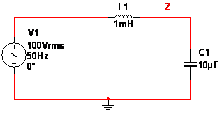
Low pass filter circuit diagram
Download Low Pass Filter Simulation
Analysis Parameters for Low pass filter
Select the Simulation and set it to Ac Sweep, set the analysis parameters
Now select the output variables meters as required in this case
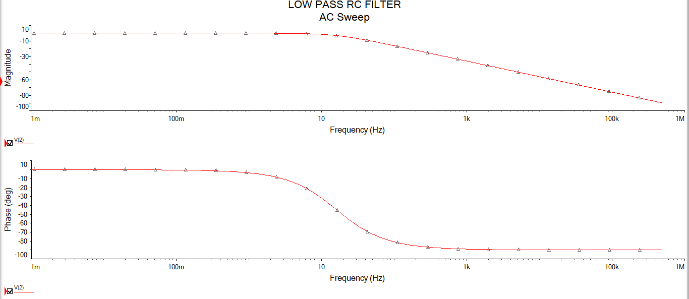
Press F5 and observe the simulation result of Circuit
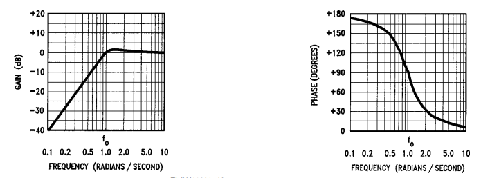
The opposite of the low-pass is the high-pass filter, which rejects signals below its cutoff frequency. A high-pass filter can be made by rearranging the components of our example network as in Figure 13. The transfer function for this filter is:
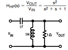
And the amplitude and phase curves are found in figure 13. Note that the amplitude response of the high-pass is a ‘‘mirror image’’ of the low-pass response. Further examples of high-pass filter responses are shown in figure 14, with the ‘‘ideal’’ response in (a) and various approximations to the ideal shown in (b) through (f). High-pass filters are used in applications requiring the rejection of low-frequency signals. One such application is in high-fidelity loudspeaker systems. Music contains significant energy in the frequency range from around 100 hz to 2 khz, but high-frequency drivers (tweeters) can be damaged if low-frequency audio signals of sufficient energy appear at their input terminals. A high-pass filter between the broadband audio signal and the tweeter input terminals will prevent low-frequency program material from reaching the tweeter. In conjunction with a low-pass filter for the low-frequency driver (and possibly other filters for other drivers), the high-pass filter is part of what is known as a ‘‘crossover network’’
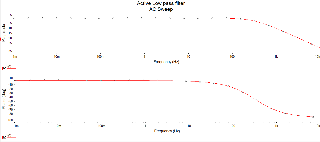
ACTIVE LOW PASS FILTER
Active filters use amplifying elements, especially op amps, with resistors and capacitors in their feedback loops, to synthesize the desired filter characteristics. Active filters can have high input impedance, low output impedance, and virtually any arbitrary gain. They are also usually easier to design than passive filters. Possibly their most important attribute is that they lack inductors, thereby reducing the problems associated with those components. Still, the problems of accuracy and value spacing also affect capacitors, although to a lesser degree. Performance at high frequencies is limited by the gain-bandwidth product of the amplifying elements, but within the amplifier’s operating frequency range, the op amp-based active filter can achieve very good accuracy, provided that low-tolerance resistors and capacitors are used. Active filters will generate noise due to the amplifying circuitry, but this can be minimized by the use of low-noise amplifiers and careful circuit design. Figure 32 shows a few common active filter configurations (There are several other useful designs; these are intended to serve as examples). The second-order Sullen-Key low pass filter can be used as a building block for higher order filters. By cascading two or more of these circuits, filters with orders of four or greater can be built. The two resistors and two capacitors connected to the op amp’s non-inverting input and to VIN determine the filter’s cutoff frequency and affect the Q; the two resistors connected to the inverting input determine the gain of the filter and also affect the Q. Since the components that determine gain and cutoff frequency also affect Q, the gain and cutoff frequency can’t be independently changed. Figures 32(b) and 32(c) are multiple-feedback filters using one op amp for each second-order transfer function. Note that each high-pass filter stage in Figure 32(b) requires three capacitors to achieve a second-order response. As with the Sallen-Key filter, each component value affects more than one filter characteristic, so filter parameters can’t be independently adjusted. The second-order state-variable filter circuit in Figure 32(d) requires more op amps, but provides high-pass, low-pass, and band pass outputs from a single circuit. By combining the signals from the three outputs, any second-order transfer function can be realized. When the center frequency is very low compared to the op amp’s gain-bandwidth product, the characteristics of active RC filters are primarily dependent on external component tolerances and temperature drifts. For predictable results in critical filter circuits, external components with very good absolute accuracy and very low sensitivity to temperature variations must be used, and these can be expensive. When the center frequency multiplied by the filter’s Q is more than a small fraction of the op amp’s gain-bandwidth product, the filter’s response will deviate from the ideal transfer function. The degree of deviation depends on the filter topology; some topologies are designed to minimize the effects of limited op amp bandwidth.
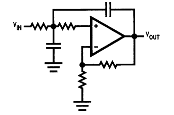
Active low pass filter circuit diagram
Wire up the Circuit as shown below.
Active Low Pass Filter Simulation
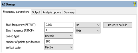
Analysis Parameters for Active low pass filter
Select the Simulation and set it to Ac Sweep, set the analysis parameters.
Press F5 and observe the simulation result of Circuit
FILTER ORDER:-
The order of a filter is important for several reasons. It is directly related to the number of components in the filter, and therefore to its cost, its physical size, and the complexity of the design task. Therefore, higher-order filters are more expensive, take up more space, and are more difficult to design. The primary advantage of a higher order filter is that it will have a steeper roll off slope than a similar lower-order filter
PASSIVE FILTERS
The filters used for the earlier examples were all made up of passive components: resistors, capacitors, and inductors, so they are referred to as passive filters. A passive filter is simply a filter that uses no amplifying elements (transistors, operational amplifiers, etc.). In this respect, it is the simplest (in terms of the number of necessary components) implementation of a given transfer function. Passive filters have other advantages as well. Because they have no active components, passive filters require no power supplies. Since they are not restricted by the bandwidth limitations of op amps, they can work well at very high frequencies. They can be used in applications involving larger current or voltage levels than can be handled by active devices. Passive filters also generate little Nosie when compared with circuits using active gain elements. The noise that they produce is simply the thermal noise from the resistive components, and, with careful design, the amplitude of this noise can be very low. Passive filters have some important disadvantages in certain applications, however. Since they use no active elements, they cannot provide signal gain. Input impedances can be lower than desirable, and output impedances can be higher the optimum for some applications, so buffer amplifiers may be needed. Inductors are necessary for the synthesis of most useful passive filter characteristics, and these can be prohibitively expensive if high accuracy (1% or 2%, for example), small physical size, or large value are required. Standard values of inductors are not very closely spaced, and it is difficult to find an off-the-shelf unit within 10% of any arbitrary value, so adjustable inductors are often used. Tuning these to the required values is time-consuming and expensive when producing large quantities of filters. Furthermore, complex passive filters (higher than 2nd-order) can be difficult and time-consuming to design.
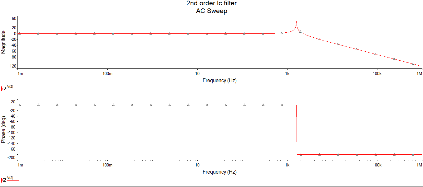
2ND ORDER LC FILTER
Second order systems are the systems or networks which contain two or more storage elements and have describing equations that are second order differential equations.
In this project great emphasis will be given on second order filters. These filters are very important for two main reasons:
- They provide an inexpensive approximation to ideal filters
- They are used as building blocks for more expensive filters that provide more accurate approximations to ideal filters.
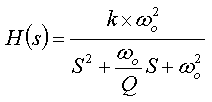
The frequency response of second order filters is characterised by three filter parameters: the gain k, the corner frequency and the quality factor Q.
A second order filter is a circuit that has a transfer function of the form:
2nd order filter circuit diagram
Wire up the Circuit as shown below.
Analysis Parameters for 2nd order filter
Select the Simulation and set it to Ac Sweep, set the analysis parameters.
Now select the output variables meters as required in this case
Press F5 and observe the simulation result of Circuit
5TH ORDER BUTTERWORTH FILTER
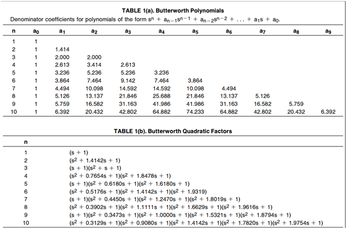
The first, and probably best-known filter approximation is the Butterworth or maximally-flat response. It exhibits a nearly flat pass band with no ripple. The roll off is smooth and monotonic, with a low-pass or high-pass roll off rate of 20 dB/decade (6 dB/octave) for every pole. Thus, a 5th-order Butterworth low-pass filter would have an attenuation rate of 100 dB for every factor of ten increase in frequency beyond the cutoff frequency. The general equation for a Butterworth filter’s amplitude response is
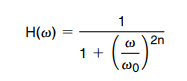
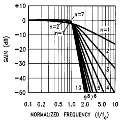
Where n is the order of the filter, and can be any positive whole number (1, 2, 3, . . . ), and 0 is the b3 dB frequency of the filter. Figure 23 shows the amplitude response curves for Butterworth low-pass filters of various orders. The frequency scale is normalized to f/fb3 dB so that all of the curves show 3 dB attenuation for f/fc e 1.0.
The coefficients for the denominators of Butterworth filters of various orders are shown in Table 1(a). Table 1(b) shows the denominators factored in terms of second-order polynomials. Again, all of the coefficients correspond to a corner frequency of 1 radian/s (finding the coefficients for a different cutoff frequency will be covered later). As an example,
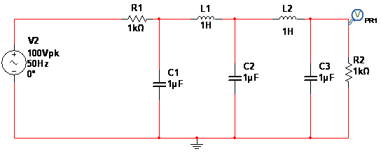
5th order Butterworth filter circuit diagram
Wire up the Circuit as shown below.
Download 5th order Butterworth Filter Simulation
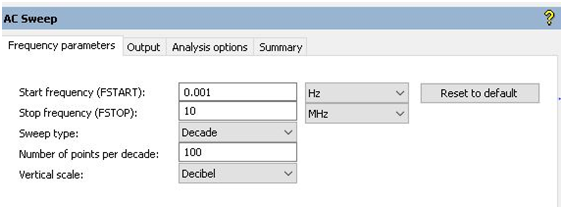
Analysis Parameters for 5th order Butterworth filter
Select the Simulation and set it to Ac Sweep, set the analysis parameters.
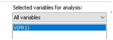
Now select the output variables meters as required in this case
Press F5 and observe the simulation result of Circuit

WHICH APPROACH IS BEST
Each filter technology offers a unique set of advantages and disadvantages that makes it a nearly ideal solution to some filtering problems and completely unacceptable in other applications. Here’s a quick look at the most important differences
ACCURACY:
Switched-capacitor filters have the advantage of better accuracy in most cases. Typical center-frequency accuracies are normally on the order of about 0.2% for most switched-capacitor ICs, and worst-case numbers range from 0.4% to 1.5% (assuming, of course, that an accurate clock is provided). In order to achieve this kind of precision using passive or conventional active filter techniques requires the use of either very accurate resistors, capacitors, and sometimes inductors, or trimming of component values to reduce errors. It is possible for active or passive filter designs to achieve better accuracy than switched-capacitor circuits, but additional cost is the penalty. A resistor-programmed switched-capacitor filter circuit can be trimmed to achieve better accuracy when necessary, but again, there is a cost penalty.
COST:
No single technology is a clear winner here. If a single-pole filter is all that is needed, a passive RC network may be an ideal solution. For more complex designs, switched-capacitor filters can be very inexpensive to buy, and take up very little expensive circuit board space. When good accuracy is necessary, the passive components, especially the capacitors, used in the discrete approaches can be quite expensive; this is even more apparent in very compact designs that require surface-mount components. On the other hand, when speed and accuracy are not important concerns, some conventional active filters can be built quite cheaply.
NOISE:
Passive filters generate very little noise (just the thermal noise of the resistors), and conventional active filters generally have lower noise than switched-capacitor ICs. Switched-capacitor filters use active op amp-based integrators as their basic internal building blocks. The integrating capacitors used in these circuits must be very small in size, so their values must also be very small. The input resistors on these integrators must therefore be large in value in order to achieve useful time constants. Large resistors produce high levels of thermal noise voltage; typical output noise levels from switched-capacitor filters are on the order of 100 mV to 300 m Vrms over a 20 kHz bandwidth. It is interesting to note that the integrator input resistors in switched-capacitor filters are made up of switches and capacitors, but they produce thermal noise the same as ‘‘real’’ resistors. (Some published comparisons of switched-capacitor vs. op amp filter noise levels have used very noisy op amps in the op amp-based designs to show that the switched-capacitor filter noise levels are nearly as good as those of the op amp-based filters. However, filters with noise levels 20 at least 20 dB below those of most switched-capacitor designs can be built using low-cost, low-noise op amps such as the LM833.) Although switched-capacitor filters tend to have higher noise levels than conventional active filters, they still achieve dynamic ranges on the order of 80 dB to 90 dB easily quiet enough for most applications, provided that the signal levels applied to the filter are large enough to keep the signals ‘‘out of the mud’’. Thermal noise isn’t the only unwanted quantity that switched-capacitor filters inject into the signal path. Since these are clocked devices, a portion of the clock waveform (on the order of 10 mV p –p) will make its way to the filter’s output. In many cases, the clock frequency is high enough compared to the signal frequency that the clock feed through can be ignored, or at least filtered with a passive RC network at the output, but there are also applications that cannot tolerate this level of clock noise.
OFFSET VOLTAGE:
Passive filters have no inherent offset voltage. When a filter is built from op amps, resistors and capacitors, its offset voltage will be a simple function of the offset voltages of the op amps and the dc gains of the various filter stages. It’s therefore not too difficult to build filters with sub-millivolt offsets using conventional techniques. Switched-capacitor filters have far larger offsets, usually ranging from a few millivolts to about 100 mV; there are some filters available with offsets over 1V! Obviously, switched-capacitor filters are inappropriate for applications requiring dc precision unless external circuitry is used to correct their offsets.
TUNABILITY:
Although a conventional active or passive filter can be designed to have virtually any center frequency that a switched-capacitor filter can have, it is very difficult to vary that center frequency without changing the values of several components. A switched-capacitor filter’s center (or cutoff) frequency is proportional to a clock frequency and can therefore be easily varied over a range of 5 to 6 decades with no change in external circuitry. This can be an important advantage in applications that require multiple center frequencies.
COMPONENT COUNT/CIRCUIT BOARD AREA:
The switched-capacitor approach wins easily in this category. The dedicated, single-function monolithic filters use no external components other than a clock, even for multiple transfer functions, while passive filters need a capacitor or inductor per pole, and conventional active approaches normally require at least one op amp, two resistors, and two capacitors per second-order filter. Resistor-programmable switched-capacitor devices generally need four resistors per second-order filter, but these usually take up less space than the components needed for the alternative approaches.
ALIASING:
Switched-capacitor filters are sampled-data devices, and will therefore be susceptible to aliasing when the input signal contains frequencies higher than one-half the clock frequency. Whether this makes a difference in a particular application depends on the application itself. Most switched-capacitor filters have clock-to-center-frequency ratios of 50:1 or 100:1, so the frequencies at which aliasing begins to occur are 25 or 50 times the center frequencies. When there are no signals with appreciable amplitudes at frequencies higher than one-half the clock frequency, aliasing will not be a problem. In a low-pass or bandpass application, the presence of signals at frequencies nearly as high as the clock rate will often be acceptable because although these signals are aliased, they are reflected into the filter’s stopband and are therefore attenuated by the filter. When aliasing is a problem, it can sometimes be fixed by adding a simple, passive RC low-pass filter ahead of the switched-capacitor filter to remove some of the unwanted high-frequency signals. This is generally effective when the switched-capacitor filter is performing a low-pass or bandpass function, but it may not be practical with high-pass or notch filters because the passive anti-aliasing filter will reduce the passband width of the overall filter response.
DESIGN EFFORT:
Depending on system requirements, either type of filter can have an advantage in this category, but switched-capacitor filters are generally much easier to design. The easiest-to-use devices, such as the LMF40, require nothing more than a clock of the appropriate frequency. A very complex device like the LMF120 requires little more design effort than simply defining the desired performance characteristics. The more difficult design work is done by the manufacturer (with the aid of some specialized software). Even the universal, resistor-programmable filters like the LMF100 are relatively easy to design with. The procedure is made even more user-friendly by the availability of filter software from a number of vendors that will aid in the design of LMF100-type filters. National Semiconductor provides one such filter software package free of charge. The program allows the user to specify the filter’s desired performance in terms of cutoff frequency, a passband ripple, stopband attenuation, etc., and then determines the required characteristics of the second-order sections that will be used to build the filter. It also computes the values of the external resistors and produces amplitude and phase vs. frequency data.